Um, Factually

# libraries
library(tidyverse)
library(riekelib)
library(patchwork)
library(gt)
library(gtExtras)

# import um actually episode-level data
actually <- 
  jsonlite::fromJSON("https://raw.githubusercontent.com/tekkamanendless/umactually/master/data.json") %>%
  map_if(is.data.frame, list) %>%
  as_tibble()

# individual contestants
people <- 
  actually %>%
  unnest(people) %>%
  select(id, name) %>%
  rowid_to_column("pid")

# pre-season 9 episodes
episodes <-
  actually %>%
  select(episodes) %>%
  unnest(episodes) %>%
  select(eid = dropouttv_productid,
         season = season_number,
         episode = number,
         players,
         questions) %>%
  filter(season <= 8)

Um, Actually: A game show of fandom minutiae one-upmanship, where nerds do what nerds do best: flaunt encyclopedic nerd knowledge at Millennium Falcon nerd-speed.

Introduction

Um, Actually is a trivia game show found on Dropout, wherein contestants are read false statements about their favorite pieces of nerdy pop culture and earn points by figuring out what’s wrong.¹ After 8 seasons, longtime host Mike Trapp and his omnipresent fact-checker Michael Salzman have relinquished their hosting and fact-checking duties. Ify Nwadiwe and Brian David Gilbert take up the mantle as host and voluntary-live-in-fact-checker in season 9.

¹ But they only get the point if they precede their correction with the phrase “um, actually…”

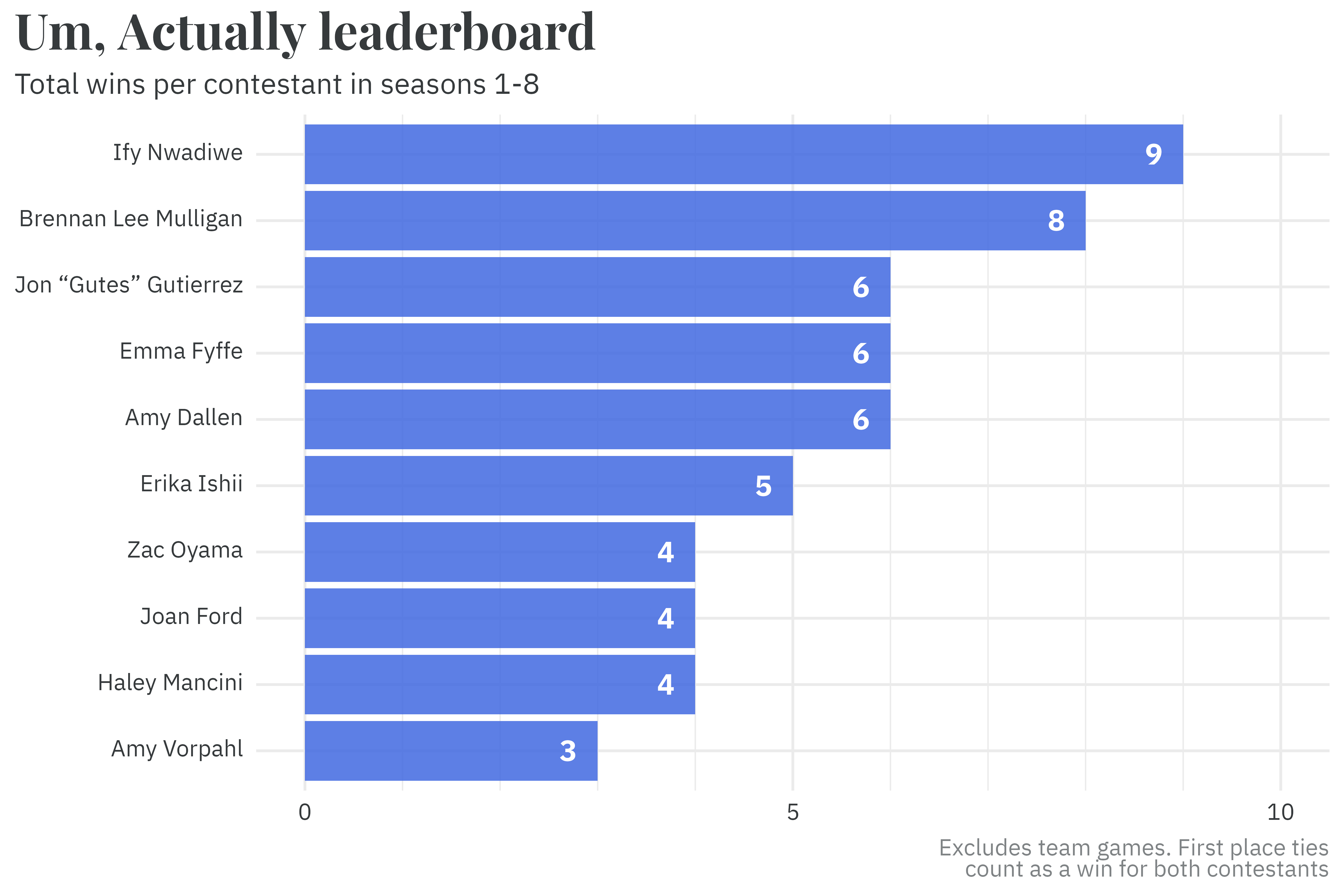
Ify’s ascendancy to host comes in the wake of an impressive run as a contestant. Ify currently holds the title of winningest contestant, with a whopping 9 total wins over the course of the first 8 seasons.

episodes %>% 
  unnest(players) %>%
  group_by(season, episode) %>%
  filter(score == max(score)) %>%
  ungroup() %>%
  count(id) %>%
  arrange(desc(n)) %>%
  left_join(people) %>%
  slice_head(n = 10) %>%
  mutate(name = fct_reorder(name, n)) %>%
  ggplot(aes(x = name,
             y = n)) + 
  geom_col(fill = "royalblue",
           alpha = 0.85) + 
  geom_text(aes(label = n),
            nudge_y = -0.3,
            family = "IBM Plex Sans",
            fontface = "bold",
            color = "white",
            size = 5) + 
  scale_y_continuous(breaks = c(0, 5, 10),
                     minor_breaks = 0:10) + 
  coord_flip() +
  theme_rieke() + 
  labs(title = "**Um, Actually leaderboard**",
       subtitle = "Total wins per contestant in seasons 1-8",
       x = NULL,
       y = NULL,
       caption = "Excludes team games. First place ties<br>count as a win for both contestants") + 
  expand_limits(y = c(0, 10))

But does winningnest contestant automatically confer the title of most skilled player? As Ify is oft lauded as the best Um, Actually player, there’s an implicit assumption that win count is the best metric for measuring player skill. But by other metrics, you might conclude that other players are better. Jared Logan, for example, has a perfect win record across three appearances on the show; Brennan Lee Mulligan has the highest proportion of points-earned to questions-asked; and Jeremy Puckett² holds the record for most points in a single game (9).³

² A fan contestant on Season 1 Episode 32

³ Ify was a contestant on this episode and received only one point.

Any proxy for player skill will have drawbacks. Win count, however, has a few specific detrimental factors that cause it to be a misleading indicator of player skill:

• contestants who appear on the show more often have more opportunities to rack up wins;
• a small 1-point win and an 8 point win both only count as one win, despite the latter being more impressive;
• whether or not a player wins depends on the relative skill of the other contestants in each game — simply tallying up wins ignores this.

A better method for measuring player skill would instead consider the points won by each contestant while taking into account the relative skill of the other players in each game. In the pedantic spirit of the game, I propose one such alternative method. By estimating latent player skill with a hierarchical Bayesian model, I uncover who, statistically, is the best Um, Actually player.

Note

If you’re just here to see the results and power ranking of each contestant, you can skip to the end. Otherwise, strap in for the cacophony of math and code used to develop the rankings.

The rules of the game

Before diving headfirst into the results or the code to generate them, it’s probably helpful to explain in detail how the game works. In each episode, three contestants vie to earn points by identifying the incorrect piece of information in a statement read by the host. Contestants buzz in to propose their corrections, which must begin with the phrase “um, actually…”. If their correction is, paradoxically, incorrect, or if they forget to say “um, actually,” the other contestants can buzz in to try to scoop the point. If no one is able to correct the host’s statement, the host reveals what was wrong and the point is lost to the ether.

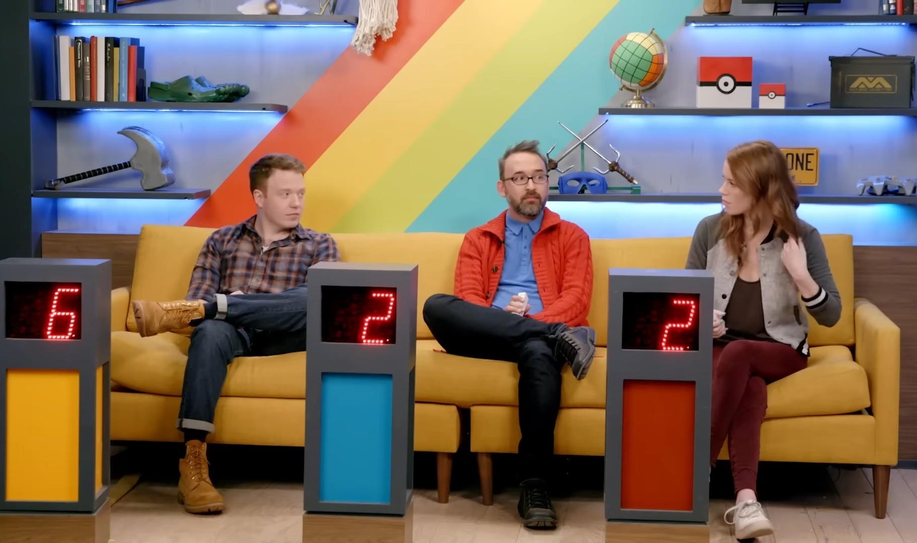
(Left to right) Brennan Lee Mulligan, Kirk Damato, and Marisha Ray as contestants — Season 2, Episode 1

Players can also scoop points by being more correct than other contestants. For example, say a player identifies the incorrect portion of the host’s statement but their correction is wrong. The host may give the other contestants a chance to scoop by correcting the correction. If the other players aren’t able to correct the correction, the first player keeps the point.

Finally, peppered throughout each episode are Shiny Questions. Shiny Questions, just like Shiny Pokémon, are worth the same amount of points, they’re just slightly different and a little rarer. Shiny Questions vary in format — sometimes contestants are tasked with identifying books based on cover alone, other times contestants must find the “fake” alien out of a group of “real” fictional aliens, and sometimes contestants try to draw cryptids accurately based on name only.

Ultimately, skilled players are those who are good at all aspects of the game. The best players not only have a deep well of niche nerd trivia knowledge, but are also quick on the buzzer, able to scoop points from other players, proficient in a wide array of mini-games in the form of Shiny Questions, and, most importantly, remember to say “um, actually.”

Um, Actually, the Model

The goal of any statistical model is to represent a stochastic process that generates data with math. Here, the observed data, the number of points won by each player in each game, is generated by unobserved differences in player skill. By working backwards through the generative process, we can link the number of points won to unobserved (latent) skill mathematically. This statistical model can then be translated to code so that we can learn the parameters of the model that maximize the probability of generating the observed data.

In each three-player game, \(g\), the number of individually awarded points that each player, \(p\), wins is modeled as a draw from a poisson distribution given the expected number of points, \(\lambda_{g,p}\). \(\lambda_{g,p}\) is simply the product of the total number of individually awarded points, \(K_g\), and player \(p\)’s probability of winning each point, \(\theta_{g,p}\).⁴

⁴ This is an example of the poisson trick — using a series of poisson likelihoods to vectorize a multinomial model.

\[ \begin{align*} R_{g,p} &\sim \text{Poisson}(\lambda_{g,p}) \\ \lambda_{g,p} &= K_g \times \theta_{g,p} \end{align*} \]

The probability of an individual player winning a point is dependent on both their skill and their skill relative to other players in the match. A highly skilled player, for example, would expect to win more points in a game with two low-skilled players than in a game with two similarly high-skilled players. Let \(\gamma_g\) be a vector containing parameters measuring latent player skill, \(\beta_p\). Applying the softmax transformation⁵ to \(\gamma_g\) converts a vector of unbounded parameters to a vector of probabilities while enforcing the constraint that \(\sum \theta_g = 1\).

⁵ \(\text{softmax}(z)_i = \frac{e^{z_i}}{\sum_j^K e^{z_j}}\)

\[ \begin{align*} \theta_g &= \text{softmax}(\gamma_g) \\ \gamma_g &= \begin{bmatrix} \beta_{p[g,1]} \\ \beta_{p[g,2]} \\ \beta_{p[g,3]} \\ 0 \end{bmatrix} \end{align*} \]

It’s worth spending more time interrogating these few lines in more detail. Firstly, sometimes no player is awarded a point. This is represented mathematically by “awarding” these points to the host at position 4 in \(\gamma\). To ensure identifiability of the players’ skill parameters, \(\beta_p\), I use the “host points” as the reference condition and fix the value to \(0\).⁶

⁶ Note that this does not mean that there is a 0% chance of awarding “host points.”

Secondly, the player in each position in \(\gamma\) can change from game to game. For example, Siobhan Thompson can appear at position 1 in one game, position 3 in another, but most often doesn’t appear at all! The model undertakes a bit of array-indexing insanity to ensure that the length of \(\gamma\) stays the same, but the player-level elements change from game to game.

Finally, although the parameter measuring player skill is static, the probability of being awarded a point can change based on the other players in the game. For example, consider a game with three equally-matched players. Unsurprisingly, they each have an equal probability of being awarded a point.

# three evenly-skilled players
beta <- c(0.5, 0.5, 0.5, 0)

# even chances of earning each point
beta %>%
  softmax() %>%
  round(2)

#> [1] 0.28 0.28 0.28 0.17

If, however, a more skilled contestant swaps in, the probability of the other players being awarded a point drops, despite their latent skill remaining the same.

# player 1 is highly skilled
beta[1] <- 1.5

# probabilities for players 2 and 3 drop
beta %>%
  softmax() %>%
  round(2)

#> [1] 0.51 0.19 0.19 0.11

Each player’s skill is modeled as hierarchically distributed around the latent skill of the average player, \(\alpha\). The hierarchical formulation allows the model to partially pool player skill estimates. Players who appear on the show many times will have relatively precise estimates of skill. Conversely, players with few appearances will tend to have skill estimates close to the average. To restrict the range of plausible values, I place standard normal priors over the parameters.

\[ \begin{align*} \beta_p &= \alpha + \eta_p \sigma \\ \alpha &\sim \text{Normal}(0, 1) \\ \eta &\sim \text{Normal}(0, 1) \\ \sigma &\sim \text{Half-Normal}(0, 1) \end{align*} \]

Breaking the rules

In most episodes, most questions follow the format described above: one of the three contestants earns a point or the point goes to no one. In these cases, the baseline model can be applied. There are, however, a few edge cases that require different model setups to accurately measure player skill.

Three-player game: multiple points awarded

About ~4% of the time in three-player games, multiple points are awarded on a single question. Most of these cases involve Shiny Questions in which players can potentially tie, but there are rare cases in which a player finds an unintendedly incorrect portion of the host’s statement and is awarded a secondary point. Regardless of the source, we’ll need to add two new components to the model to account for this:

• a method for estimating the number of points awarded per question, and
• a method for connecting the observed data (points awarded) to player skill when multiple points are awarded.

How many points were awarded?

Estimating the number of points awarded per question is the easier of the two tasks, so we’ll start there. Let \(S_g\) be a vector with three elements that counts the number of questions in each game, \(g\), in which the point was awarded to one player (or no one), two players, or all three players. We can model it as a draw from a multinomial distribution where \(K_g\) is the number of questions in each game and \(\phi\) is a vector of probabilities corresponding to each category in \(S\).

\[ \begin{align*} S_g &\sim \text{Multinomial}(K_g, \phi) \\ \phi &= \begin{bmatrix} \phi_1 \\ \phi_2 \\ \phi_3 \end{bmatrix} \\ \end{align*} \]

The categories in \(S\) are ordinal — one point is less than two points is less than three. To enforce an ordinal outcome, the probabilities in \(\phi\) are generated by dividing the range \([0,1]\) into three \(\phi\)-sized regions with two cutpoints, \(\omega\).⁷ The model just needs to determine the values of \(\omega\). Applying the logit transform to \(\omega\) yields the unbounded \(\kappa\), over which I place a \(\text{Normal}(0,1.5)\) prior.⁸

⁷ For a detailed introduction to modeling ordinal outcomes, see Chapter 12 Section 3 of Statistical Rethinking by Richard McElreath. I also cover ordinal models in more detail here.

⁸ In code, I enforce the consistent ordering of \(\kappa_2 > \kappa_1\) with Stan’s ordered data type.

\[ \begin{align*} \phi_1 &= \omega_1 \\ \phi_2 &= \omega_2 - \omega_1 \\ \phi_3 &= 1 - \omega_2 \\ \text{logit}(\omega_k) &= \kappa_k \\ \kappa &\sim \text{Normal}(0, 1.5) \end{align*} \]

So you’re saying there’s a chance?

Modeling the case in which two players are awarded a point on a single question is a bit involved. If two points are awarded on a single question, \(q\), in game \(g\), whether (or not) each individual player \(p\) is awarded one of the possible points can be modeled as a draw from a bernoulli distribution with probability \(\Theta_{g,p}\).⁹

⁹ This can be alternatively modeled at the game level as a draw from a binomial distribution.

\[ \begin{align*} R_{g,p,q} &\sim \text{Bernoulli}(\Theta_{g,p}) \end{align*} \]

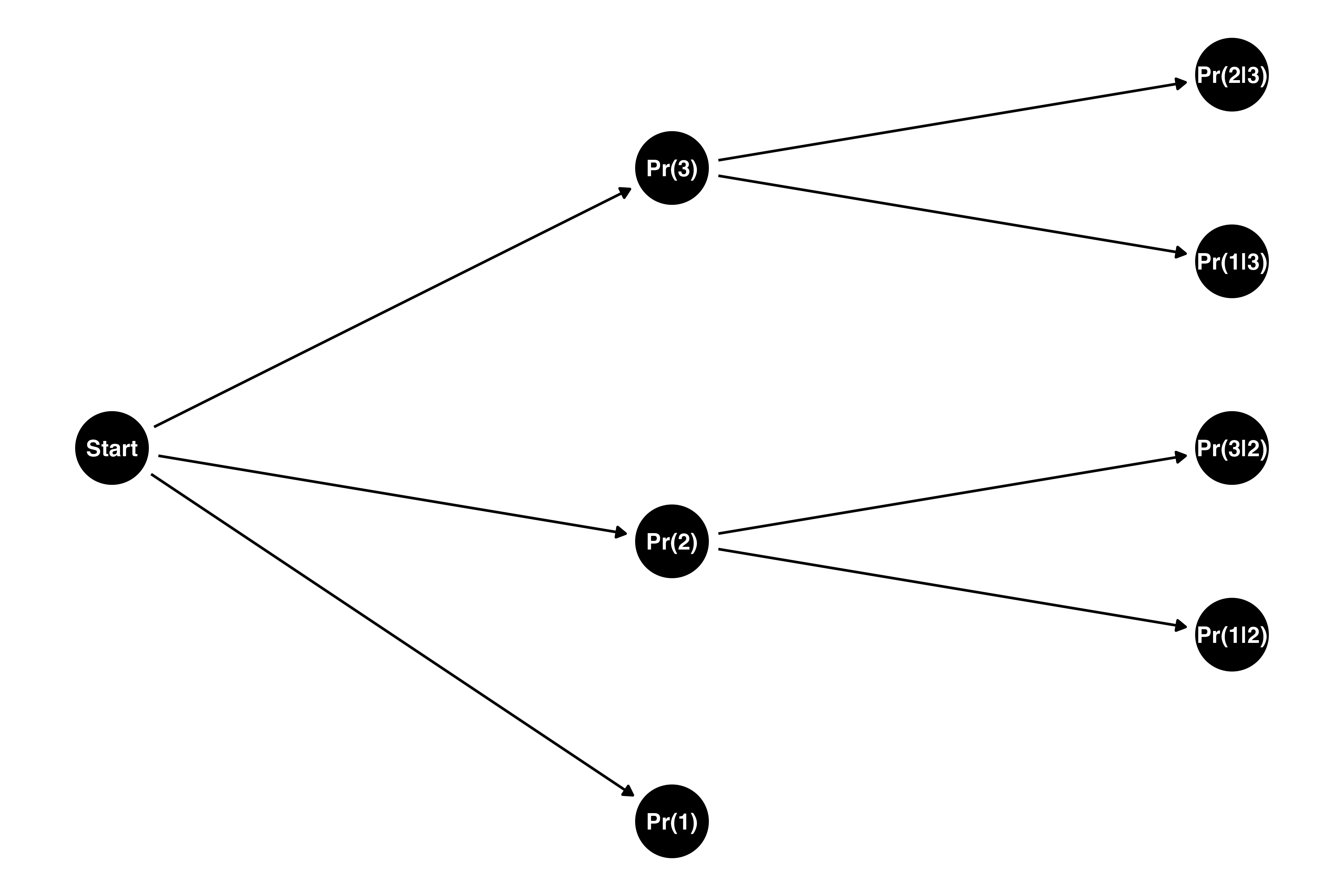
Since two points are awarded, \(\Theta_{g,p}\) represents something distinctly different from \(\theta_{g,p}\) and must be estimated differently.¹⁰ Although points are awarded simultaneously, rather than sequentially, it’s useful in this case to think of the possible outcomes as belonging to a garden of forking paths — each path we choose at each fork in the garden represents a different possible reality. Let’s look at player 1, specifically — all possible realities of two points being awarded follow one of the sequences below.

¹⁰ Notably, since two points are awarded, \(\sum \Theta_g = 2\).

dagitty::dagitty("dag {
  Start -> Po1
  Start -> Po2
  Start -> Po3
  Po2 -> P21
  Po2 -> P23
  Po3 -> P31
  Po3 -> P32
}") %>%
  ggdag::tidy_dagitty(layout = "partition") %>%
  mutate(name = case_match(name,
                           "Po1" ~ "Pr(1)",
                           "Po2" ~ "Pr(2)",
                           "Po3" ~ "Pr(3)",
                           "P21" ~ "Pr(1|2)",
                           "P23" ~ "Pr(3|2)",
                           "P31" ~ "Pr(1|3)",
                           "P32" ~ "Pr(2|3)",
                           .default = name)) %>%
  ggdag::ggdag(parse = TRUE) +
  scale_color_identity() + 
  coord_flip() +
  theme_void()

Each of these sequences occurs with some probability. The first point, for example, can be awarded to player 1, 2, or 3. The probability that the first point is awarded to each player, then, is simply \(\theta_{g,p}\).¹¹

¹¹ I’m being a bit loose with notation here as I’m running out of greek letters — this is slightly different from the \(\theta_{g,p}\) in the base model. Estimating this \(\theta_{g,p}\) is explained in detail later.

\[ \begin{align*} \Pr(1) &= \theta_{g,1} \\ \Pr(2) &= \theta_{g,2} \\ \Pr(3) &= \theta_{g,3} \\ \end{align*} \]

If the first point is awarded to player 1, we don’t need to know where the second point goes, and the diagram ends at the first node. If the first point instead is awarded to, say, player 2, then the second point can either be awarded to player 1 or player 3. The probability of player 1 winning the point conditional on the first point having been awarded to player 2 is player 1’s chances of winning relative to player 3.

\[ \begin{align*} \Pr(1 | 2) &= \frac{\theta_{g,1}}{\theta_{g,1} + \theta_{g,3}} \end{align*} \]

To get the probability of the sequence occurring, we just need to multiply by the probability of player 2 being awarded the first point.

\[ \begin{align*} \Pr(2 \rightarrow 1) &= \theta_{g,2} \frac{\theta_{g,1}}{\theta_{g,1} + \theta_{g,3}} \end{align*} \]

\(\Theta_{g,1}\) is the sum of all possible paths that lead to player 1 being awarded a point. So, repeating the process for the path where player 3 is awarded the first point yields the following:

\[ \begin{align*} \Theta_{g,1} &= \Pr(1) + \Pr(2 \rightarrow 1) + \Pr(3 \rightarrow 1) \\ &= \theta_{g,1} + \theta_{g,2}\frac{\theta_{g,1}}{\theta_{g,1} + \theta_{g,3}} + \theta_{g,3}\frac{\theta_{g,1}}{\theta_{g,1} + \theta_{g,2}} \end{align*} \]

This gets to the fundamental idea, but can be reduced with some algebra and a bit of notation. It’s helpful to first factor out \(\theta_{g,1}\).

\[ \begin{align*} \Theta_{g,1} &= \theta_{g,1} \left(1 + \frac{\theta_{g,2}}{\theta_{g,1} + \theta_{g,3}} + \frac{\theta_{g,3}}{\theta_{g,1} + \theta_{g,2}}\right) \end{align*} \]

Notice here that \(\theta_{g,1}\), \(\theta_{g,2}\), and \(\theta_{g,3}\) all appear in both fractions, but the positions change. The sum in the denominator always excludes the value in the numerator, so we can write the denominator as \(\sum \theta_{g,-j}\), where \(\theta_{g,j}\) is the value that appears in the numerator. Notice also that \(\theta_{g,1}\) never appears in the numerator and always appears in the denominator. We can enforce this notationally by indicating that \(j \neq p\) in the summation.

\[ \begin{align*} \Theta_{g,p} &= \theta_{g,p} \left(1 + \sum_{j \neq p} \frac{\theta_{g,j}}{\sum \theta_{g,-j}} \right) \end{align*} \]

Just like the single-point case, \(\theta_{g,p}\) can be connected to the parameters measuring latent skill, \(\beta_p\), via a softmax transformation. The one difference is that the reference condition for the host is excluded — for all cases in which two points are awarded, there are no “host points!”

\[ \begin{align*} \theta_g &= \text{softmax}(\gamma_g) \\ \gamma_g &= \begin{bmatrix} \beta_{p[g,1]} \\ \beta_{p[g,2]} \\ \beta_{p[g,3]} \end{bmatrix} \end{align*} \]

You get a point! You get a point! You get a point!

When all three players are awarded a point on a question, there is quite literally no additional work to do! If every player is awarded a point, the probability that each individual earns a point is \(1\). All of the modeling work is handled implicitly when estimating the probability that \(S_{g,q}[3] = 1\).

\[ \begin{align*} (\theta_{g,p,q}\ |\ S_{g,q}[3] = 1) &= 1 \end{align*} \]

The four player game

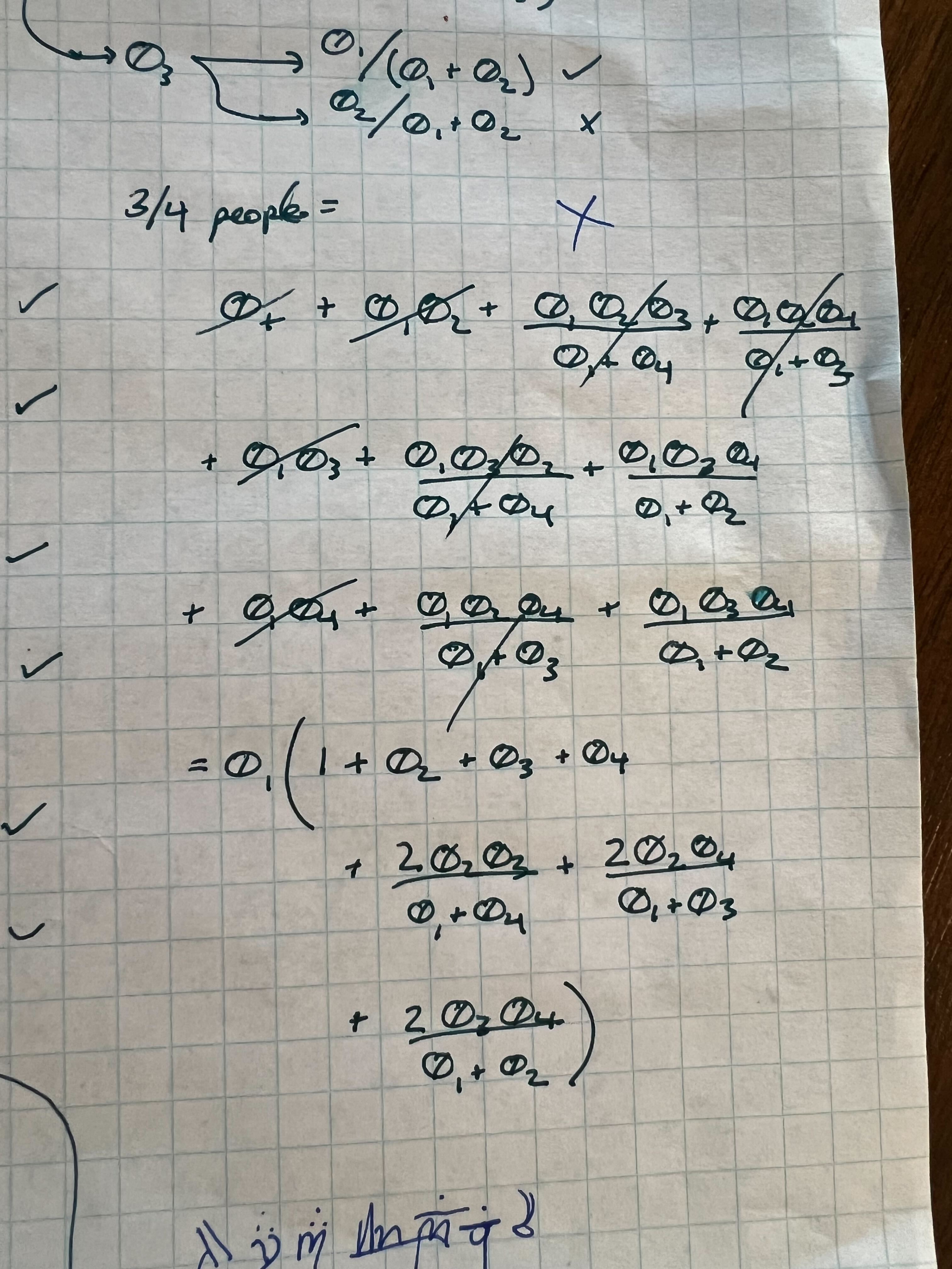
At New York’s Comic Con in 2019, Mike Trapp hosted a live episode¹² of Um, Actually with a fan, Jamel Wood, as a fourth contestant. Although players could potentially be awarded multiple points per question, this didn’t happen. Thankfully, the model doesn’t need to account for the possibility of multiple players being awarded points on a single question in a four-player game.¹³ It does, however, need to accommodate the four-person structure.

¹² Season 2, episode 11

¹³ The math to estimate this is an even clunkier mess of algebra than the case of two points awarded in a three-player game:

Mike Trapp as host for a live episode of Um, Actually at New York Comic Con in 2019 — Season 2, Episode 11

The setup is nearly identical to the base case of a three-player game. The only difference is that the vectors \(\theta_g\) and \(\gamma_g\) now include an additional element to accommodate the fourth player.

\[ \begin{align*} R_{g,p} &\sim \text{Poisson}(\lambda_{g,p}) \\ \lambda_{g,p} &= K_g \times \theta_{g,p} \\ \theta_g &= \text{softmax}(\lambda_g) \\ \gamma_g &= \begin{bmatrix} \beta_{p[g,1]} \\ \beta_{p[g,2]} \\ \beta_{p[g,3]} \\ \beta_{p[g,4]} \\ 0\end{bmatrix} \end{align*} \]

Team games

Three regular-season episodes¹⁴ break from the three-player format and instead pitch two teams of two players against each other. Like three-player games, multiple points per question can be awarded in team games. Again, we’ll need to add two components to the model:

¹⁴ Season 3, episode 2, season 5, episodes 1 and 21.

• a method for estimating the number of points awarded per question, and
• a method for connecting the observed data (points awarded) to player skill based on the number of awarded points.

How many points were awarded?

In each team game, \(g\), the number of questions with points awarded to both teams, \(S_g\), is modeled as a draw from a binomial distribution where \(K_g\) is the number of questions in each game and \(\delta\) is the probability that points are awarded to both teams. This is a relatively rare occurrence, so I place an informative prior over \(\text{logit}(\delta)\).

\[ \begin{align*} S_g &\sim \text{Binomial}(K_g, \delta) \\ \text{logit}(\delta) &\sim \text{Normal}(-2,0.5) \end{align*} \]

One team, two team, red team, blue team

The case where one team is awarded a point is very similar to the base case of a three-player game. The number of individually-awarded points each team, \(t\), earns is modeled as a draw from a poisson distribution given an expected number of points, \(\lambda_{g,t}\), which is the product of the total number of points to be awarded, \(K_g\), and team \(t\)’s probability of winning a point, \(\theta_{g,t}\).

\[ \begin{align*} R_{g,t} &\sim \text{Poisson}(\lambda_{g,t}) \\ \lambda_{g,t} &= K_g \times \theta_{g,t} \end{align*} \]

I assume that individual player skill contributes directly to the overall team skill. Therefore, \(\theta_g\) and \(\gamma_g\) differ slightly from the base three-player variants in two important ways:

• each vector is one element shorter since they only need to account for two teams rather than three players, and
• team skill is estimated as the sum of players’ skill within the team.

\[ \begin{align*} \theta_g &= \text{softmax}(\gamma_g) \\ \gamma_g &= \begin{bmatrix} \beta_{p[g,1]} + \beta_{p[g,2]} \\ \beta_{p[g,3]} + \beta_{p[g,4]} \\ 0 \end{bmatrix} \end{align*} \]

Points across the board

Much like the three-player game, when both teams are awarded a point on a question, there is no additional work to do, since the probability that each individual team earns a point is \(1\). All the modeling work is handled implicitly during the estimation of \(S_{g,q}=1\).¹⁵

¹⁵ For clarity, \(S_{g,q}=1\) here indicates that both teams were awarded a point and \(S_{g,q}=0\) indicates that one or zero teams were awarded a point.

\[ \begin{align*} (\theta_{g,t,q}\ |\ S_{g,q} = 1) &= 1 \end{align*} \]

Results

To recap, the goal of this model is to determine who the best Um, Actually player is in terms of player skill. Player skill is evaluated by modeling the number of points won by each player while considering the relative skill of the other players in each game. Edge cases, like multiple points being awarded for a single question, team games, and four-player games, require slightly different setups to link the outcome to latent skill, but the overall idea remains the same. The model is fit using Stan — the source code can be found in the repository for this post.

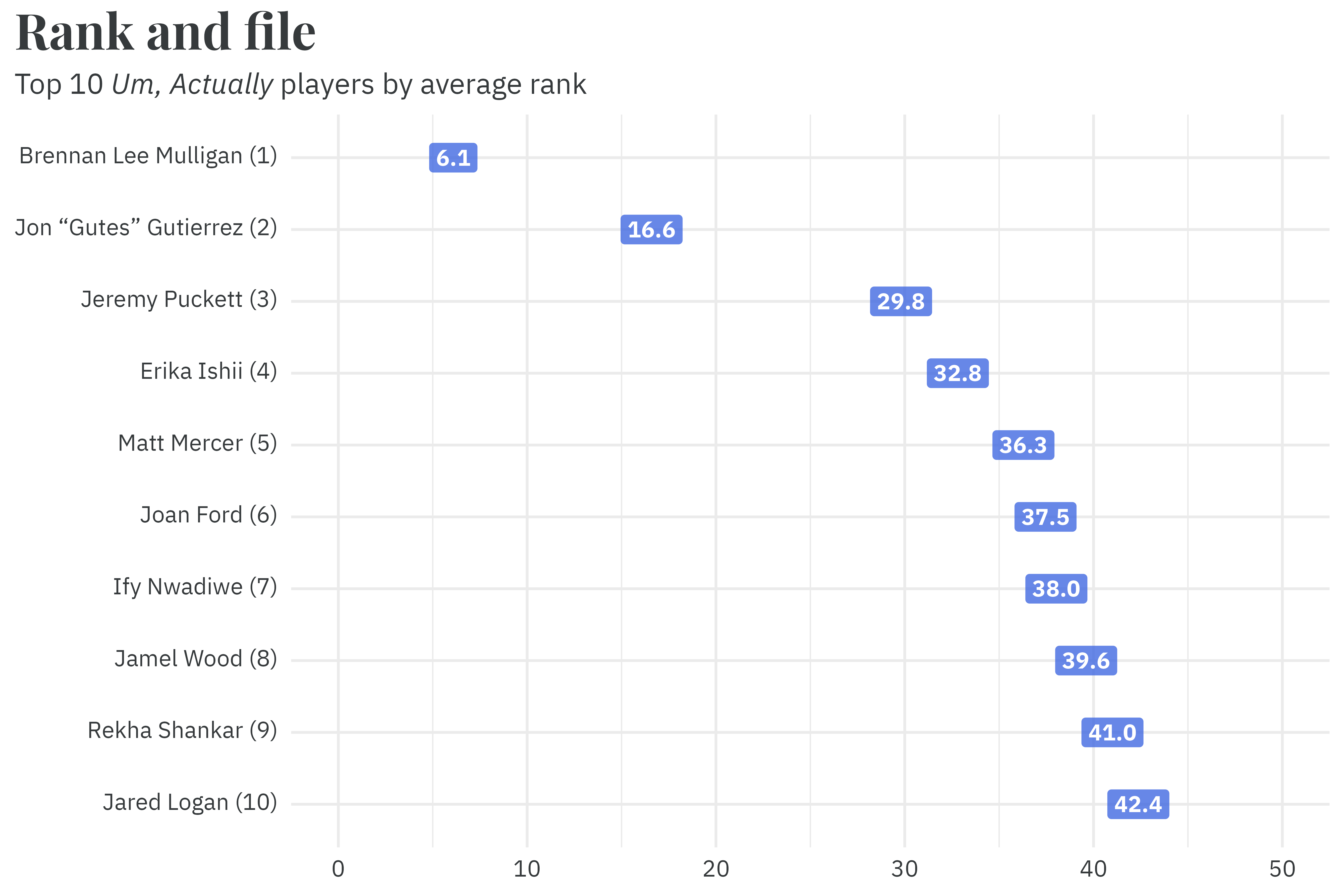
In each of the model’s simulations, the skill estimates are ranked in descending order. The average rank is, unsurprisingly, the average across all of the model’s simulations. By this method, the model finds Brennan Lee Mulligan to be the best Um, Actually player, with an average skill rank of 6.1. Ify Nwadiwe, despite having the most wins, is considered to be the 7th best contestant, with an average skill rank of 38.0.

avg_rank <-
  read_csv("out/avg_rank.csv")

alpha <-
  read_csv("out/alpha.csv") %>%
  pull(mean)

avg_rank %>%
  arrange(rank) %>%
  slice_head(n = 10) %>%
  mutate(name = glue::glue("{name} ({rank})"),
         name = fct_reorder(name, -rank),
         label = scales::label_number(accuracy = 0.1)(rank_score)) %>%
  ggplot(aes(x = name,
             y = rank_score,
             label = label)) + 
  geom_label(label.size = 0,
             color = "white",
             fill = "royalblue",
             alpha = 0.8,
             family = "IBM Plex Sans",
             fontface = "bold") + 
  coord_flip() +
  theme_rieke() +
  labs(title = "**Rank and file**",
       subtitle = "Top 10 *Um, Actually* players by average rank",
       x = NULL,
       y = NULL) +
  expand_limits(y = c(0, 50))

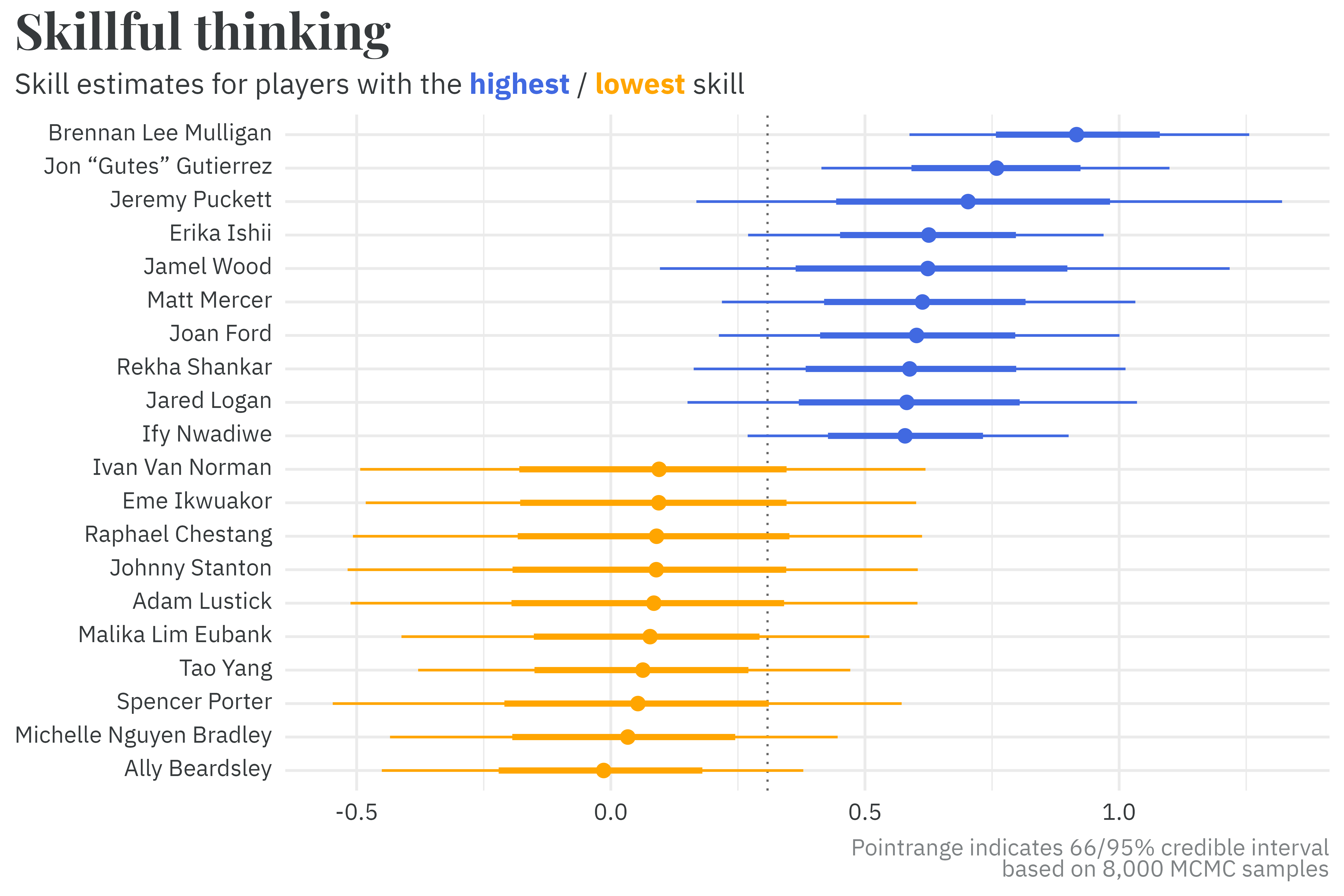
Average rank is an appropriate summary, but it’s useful to look at the full distribution of each player’s skill estimate to get a better sense of the uncertainty in this measurement. Most players have appeared on the the show fewer than ten times, leading to relatively imprecise estimates for player skill. Even among the most/least skilled players, the uncertainty intervals often include the average player skill!¹⁶

¹⁶ The average player has a skill value of about 0.31 (the dotted line in the chart below).

player_skill <- 
  read_csv("out/player_skill.csv")
  
top_players <- 
  player_skill %>%
  nest(data = -c(name, estimate)) %>%
  arrange(desc(estimate)) %>%
  slice_head(n = 10)

bottom_players <-
  player_skill %>%
  nest(data = -c(name, estimate)) %>%
  arrange(estimate) %>%
  slice_head(n = 10)
top_players %>%
  mutate(color = "royalblue") %>%
  bind_rows(bottom_players %>% mutate(color = "orange")) %>%
  unnest(data) %>%
  mutate(name = fct_reorder(name, estimate)) %>%
  ggplot(aes(x = name,
             y = estimate,
             ymin = .lower,
             ymax = .upper,
             .width = .width,
             color = color)) + 
  geom_hline(yintercept = alpha,
             linetype = "dotted",
             color = "gray40") + 
  ggdist::geom_pointinterval() +
  scale_color_identity() + 
  coord_flip() +
  theme_rieke() +
  labs(title = "**Skillful thinking**",
       subtitle = glue::glue("Skill estimates for players with the ",
                             "**{color_text('highest', 'royalblue')}** / ",
                             "**{color_text('lowest', 'orange')}** skill"),
       x = NULL,
       y = NULL,
       caption = paste("Pointrange indicates 66/95% credible interval",
                       "based on 8,000 MCMC samples",
                       sep = "<br>"))

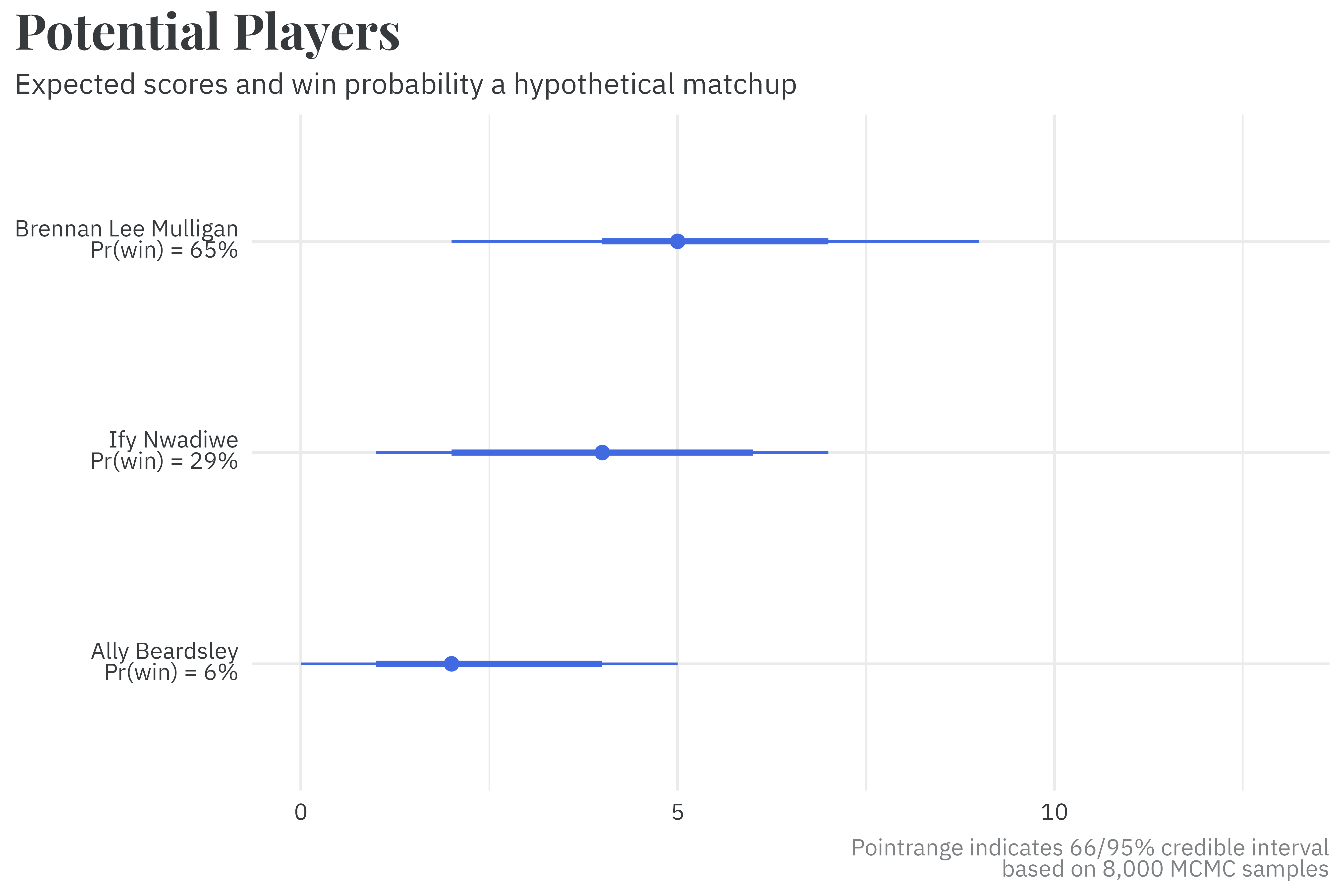
Uncertainty in the skill estimates means that, even when there is a large skill difference between players, the low-skilled players still have an outside chance of winning in a standard 13-question/three-player game. For example, consider a hypothetical matchup between two highly skilled players, Brennan Lee Mulligan and Ify Nwadiwe, and a low-skill player, Ally Beardsley. Brennan is expected to win the most points and has the highest probability of winning,¹⁷ but Ally still is expected to win a few points. They also have a low, but not impossible, chance of winning!

¹⁷ This is estimated including the possiblity of multiple points being awarded per question. In the even of a tie, players with the top score share the win.

win_probs <- 
  tibble(file = list.files("out/")) %>%
  filter(str_sub(file, 1, 4) == "prob",
         !str_detect(file, "prob_best")) %>%
  mutate(prob = map(file, ~read_csv(paste0("out/", .x)))) %>%
  unnest(prob)

games <- 
  tibble(file = list.files("out/")) %>%
  filter(str_detect(file, "score")) %>%
  mutate(scores = map(file, ~read_csv(paste0("out/", .x)))) %>%
  unnest(scores) %>%
  select(-file) %>%
  left_join(win_probs) %>%
  nest(data = -file) %>%
  rowid_to_column("game") %>%
  mutate(game = paste("Game", game)) %>%
  unnest(data) %>%
  mutate(name = glue::glue("{name}<br>Pr(win) = {scales::label_percent(accuracy = 1)(p_win)}"))

plot_game <- function(gid) {
  
  games %>% 
    filter(str_detect(game, as.character(gid))) %>%
    mutate(name = fct_reorder(name, p_win)) %>%
    ggplot(aes(x = name,
               y = score,
               ymin = .lower,
               ymax = .upper,
               .width = .width)) + 
    ggdist::geom_pointinterval(color = "royalblue") +
    coord_flip() +
    theme_rieke() +
    expand_limits(y = c(0, 13)) +
    labs(title = "**Potential Players**",
         subtitle = "Expected scores and win probability a hypothetical matchup",
         x = NULL,
         y = NULL,
         caption = paste("Pointrange indicates 66/95% credible interval",
                         "based on 8,000 MCMC samples",
                         sep = "<br>"))
  
} 

plot_game(4)

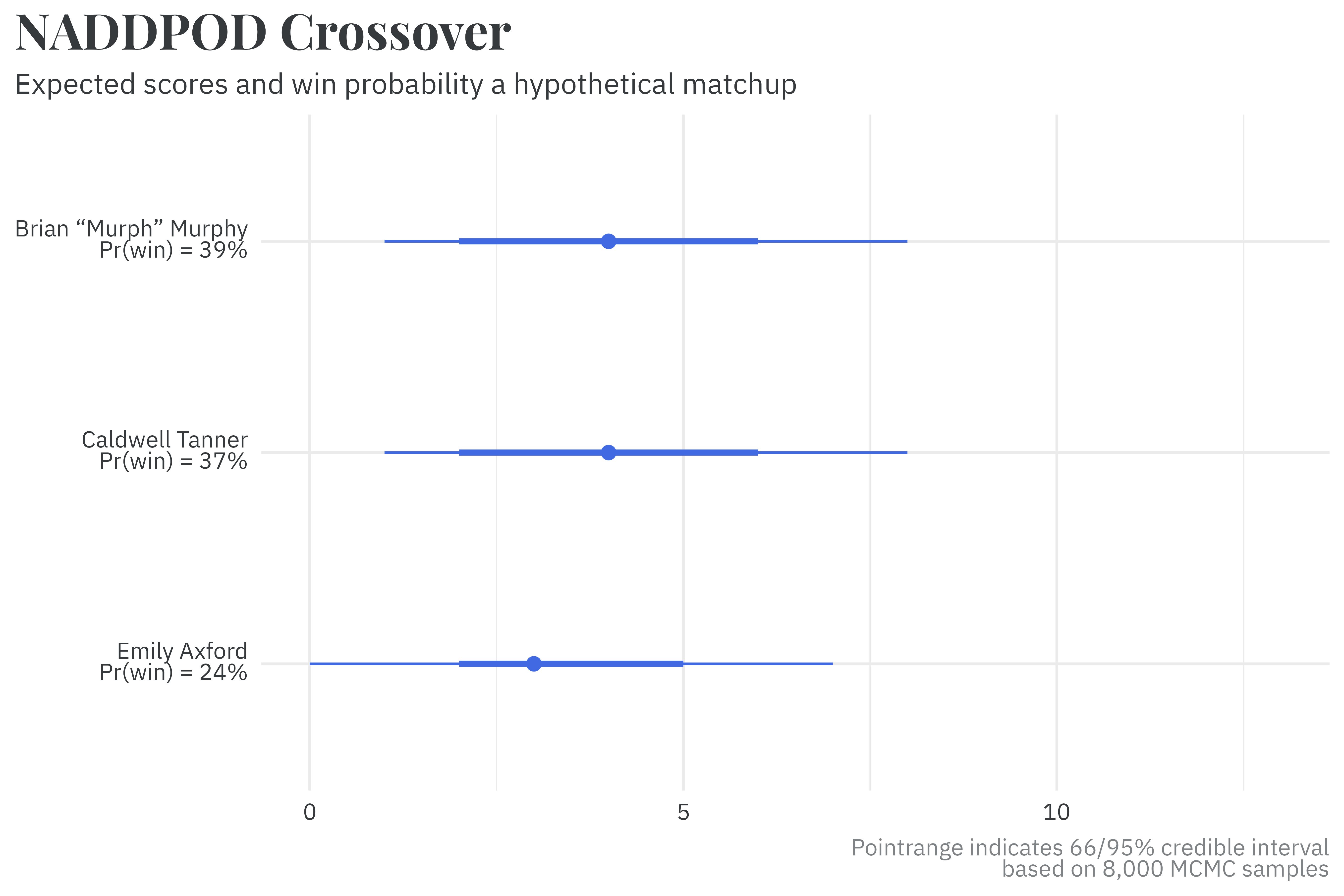
In a hypothetical matchup between more evenly matched players, the projected scores and probabilities of winning are much closer to one another. If the cast of NADDPOD¹⁸ were to face each other, Brian Murphy and Caldwell Tanner would expect to score about the same on average, but there’s a very good chance that Emily Axford produces an upset win.

¹⁸ Jake Hurwitz has yet to appear on Um, Actually, so the model would consider him to have the skill of an average player.

plot_game(2) +
  labs(title = "**NADDPOD Crossover**")

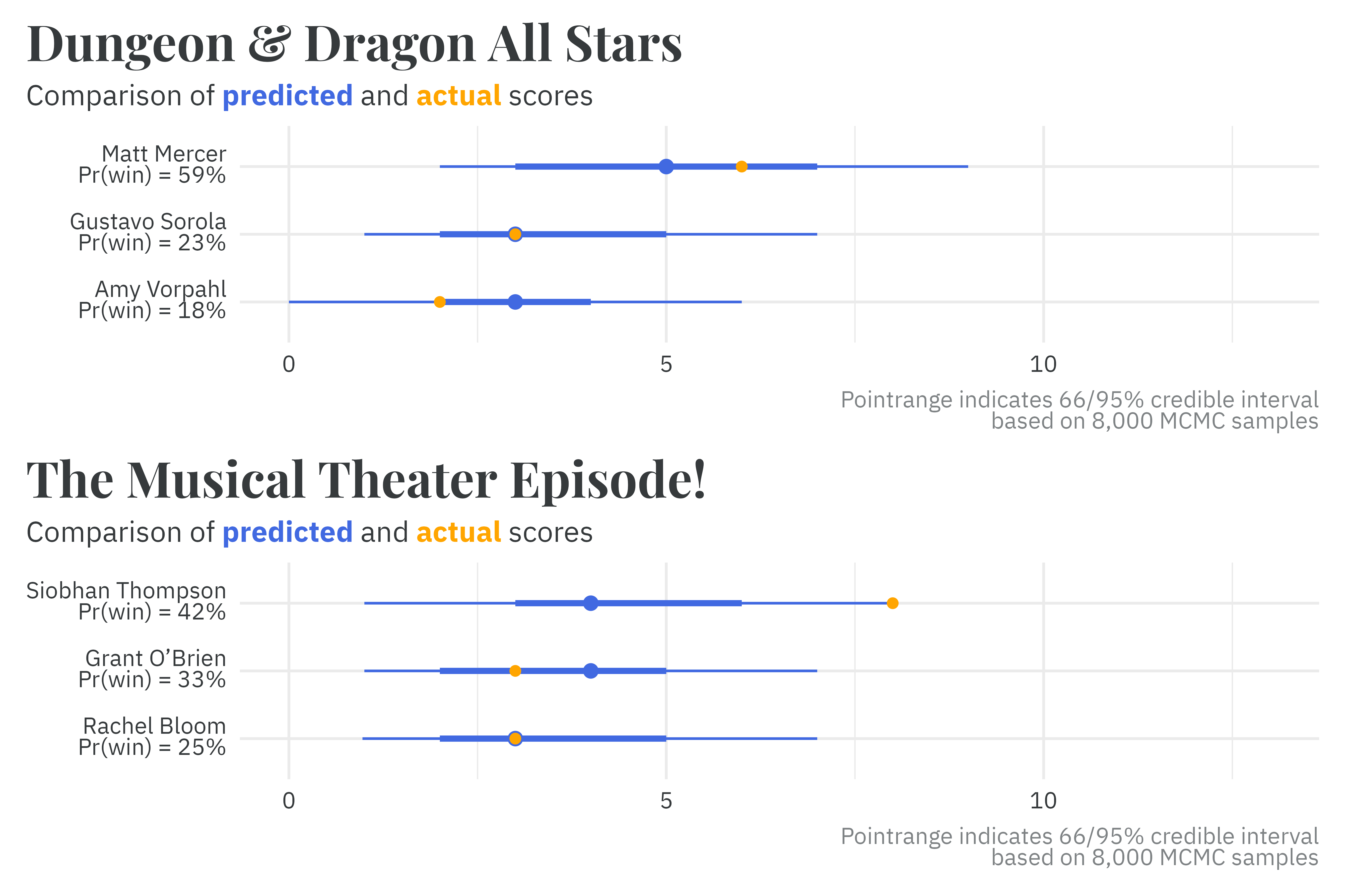
We can also compare the model predictions to the actual outcomes in specific games.¹⁹ Season 4, episode 5 was a DnD themed episode pitting three dungeon master contestants against one another. In Season 2, episode 7, three dramatic connoisseurs faced off to flex their musical theater trivia knowledge.

¹⁹ In an ideal world, I’d have compared posterior predictions for all games. This would require a good chunk of additional coding work, so you’re just gonna have to live with these few examples for the time being.

p1 <- 
  plot_game(1) + 
   geom_point(data = tibble(x = 1:3,
                            y = c(2, 3, 6)),
              mapping = aes(x = x,
                            y = y,
                            ymin = NULL,
                            ymax = NULL,
                            .width = NULL),
              color = "orange",
              size = 2) +
   labs(title = "**Dungeon & Dragon All Stars**",
        subtitle = glue::glue("Comparison of **{color_text('predicted', 'royalblue')}** ",
                              "and **{color_text('actual', 'orange')}** scores"))

p2 <- 
  plot_game(3) +
  geom_point(data = tibble(x = 1:3,
                           y = c(3, 3, 8)),
             mapping = aes(x = x,
                           y = y,
                           ymin = NULL,
                           ymax = NULL,
                           .width = NULL),
             color = "orange",
             size = 2) +
  labs(title = "**The Musical Theater Episode!**",
       subtitle = glue::glue("Comparison of **{color_text('predicted', 'royalblue')}** ",
                              "and **{color_text('actual', 'orange')}** scores"))

p1 / p2

In conclusion, the methodology presented here represents an opinionated manner of evaluating player skill that improves upon the simple method of counting total wins. This model can be used to simulate the potential outcomes of hypothetical games to see which games would produce blowout wins or tight contests. As more episodes are released, player skill estimates can be updated to produce up-to-date rankings of the best Um, Actually players.

This work would not be possible without the work of Doug Manley, who maintains umactually.info, a site containing summary statistics for every question in every game of Um, Actually.

Um, Actually Power Rankings